Rhythmic Regularity Beyond Meter and Isochrony
Jason Yust
| PDF | CITATION | AUTHOR |
Abstract
Classical meter theory, derived from European, notation-based musical practice, requires notionally absolute isochrony. This article proposes a more flexible concept of rhythmic frequencies (or periodicities) represented by continuous functions over time, and develops rhythmic theory from it that is more global in scope. A rhythm is a good fit to a given frequency if its onsets are close to peaks of one of these functions, without having to precisely coincide. This provides some useful tools for understanding properties of rhythms and how different rhythms interact, including the rhythmic spectrum which shows all the frequencies present in a rhythm. Maximally even rhythms like the African standard pattern and tamborim rhythm of samba, are those which maximize a given frequency for a given grid, and often function as basic rhythms (e.g. “timelines” or claves) in many musical traditions, as do other rhythms, like the “Bo Diddley” rhythm and Clave Son, with strong representation of a single frequency. When rhythms expressing nearby frequencies are combined, they interact to produce slow phase shifts over longer cycles, a feature of timeline rhythms, and also more complex isorhythmic designs in, for example, the late music of György Ligeti, and recent jazz compositions by Dave King and Miles Okazaki.
Keywords: clave; Fourier transform; György Ligeti; maximal evenness; meter theory; Miles Okazaki; polyrhythm; timeline rhythms.
Résumé
La théorie métrique classique, issue de la pratique musicale européenne fondée sur la notation, implique la notion d’une isochronie absolue. Cet article propose une conception plus souple des fréquences rythmiques (ou périodicités), représentées par des fonctions continues dans le temps, de manière à développer une théorie rythmique plus large dans sa portée. Un rythme s’accorde bien avec une fréquence donnée si ses attaques se situent à proximité des pics de l’une de ces fonctions, sans devoir nécessairement coïncider de façon exacte. Cette approche offre des outils utiles pour comprendre les propriétés des rythmes ainsi que la manière dont différents rythmes interagissent, notamment le spectre rythmique, qui montre l’ensemble des fréquences présentes dans un rythme. Les rythmes optimalement répartis, tels que le « rythme africain standard » (African standard pattern) ou le rythme de tamborim dans la samba, sont ceux qui maximisent une fréquence donnée pour une grille donnée, et servent souvent de rythmes fondamentaux (par exemple, des « timelines » ou des claves) dans de nombreuses traditions musicales. Il en va de même pour d’autres rythmes, tels que le « rythme Bo Diddley » ou la clave son, caractérisés par une forte représentation d’une fréquence unique. Lorsque des rythmes exprimant des fréquences proches sont combinés, ils interagissent pour produire de lents déphasages sur des cycles plus longs – une caractéristique des rythmes timeline – ainsi que des conceptions isorythmiques plus complexes que l’on trouve, par exemple, dans les dernières œuvres de György Ligeti et dans certaines compositions récentes de Dave King et Miles Okazaki.
Mots clés : György Ligeti ; Miles Okazaki ; polyrythmie ; maximal evenness ; rythmes timeline ; théorie métrique ; transformée de Fourier.
Notation, Meter, and the Concept of Rhythm
When we talk or write about rhythm, we are likely to take for granted that we know what the object of study, rhythm, is. We usually treat it, for example, as a kind of musical parameter having to do with the placement of notes in time, and which can be independently abstracted from timbre and pitch. This is very clear in musical notation, which uses an independent array of symbols for indicating timepoints of attack and release. However, we imagine also that rhythm describes a property of sound and of musical actions, and there it is not immediately apparent that the separation of parameters is so straightforward. Rhythm also involves ideas of regularity and patterning, which we capture by giving a concept of meter a prominent place in our understanding of rhythm. Our conceptualization of meter is highly determined by the European music notational system and the formal properties of its system of rhythmic symbols. These habits are so engrained that they feel natural, and it is hard to achieve a perspective from which we can question and critique them. But it is not automatic that the formal system for notating rhythms also adequately describes rhythm as a property of sound, musical action, or the mental representations of a musical participant. The notational system is designed as a prescriptive tool, optimized to instruct musicians in how to play a particular piece (Seeger 1958). Theorists and musicologists use notation as a descriptive tool, a task for which it is not designed. If the requirements of notation as a prescriptive tool conflict with this descriptive function, the design will favour the prescriptive function.
The purpose of this article is to propose a way of viewing rhythm in frequency space that gives us new way of looking at pattern and regularity in rhythm, freed from some of the implicit features of the traditional concept of meter. I begin by observing some of the descriptive inadequacies of the European notational system, focusing especially on the feature of time discreteness. A natural reaction to this shortcoming is to retrofit standard notation with “microtiming deviations.” The flaw of time discreteness however is not just one of descriptive adequacy, but also that it leads to problematically time-discrete conceptions of meter. I therefore propose a time-continuous conception of meter based on simple periodic functions. In this theory “microtiming” or “expressive timing” are not categorically distinguished from rhythm and meter, but affect rhythm and meter at a different place in the frequency continuum than the kinds of differences more commonly reflected in standard notation. I go on to develop tools from this model—spectra and two-dimensional frequency spaces—and show how these can reveal aspects of maximally even rhythms, microrhythm, and interactions of neighbouring periodicities that are intractable from the traditional time-discrete perspective. These tools have been described before (Amiot 2016; Yust 2021a–b) but I explain them from a somewhat different starting point here, in order to emphasize theoretical aspects important to the topic of meter.
To be clear, however, my critique of notation-based theories of meter here is not a broad totalizing critique of the use of notation as a descriptive tool. There is a strong history in ethnomusicology, for instance, of critiquing transcription using European notation as a perpetuation of colonialist practices (Marian-Blasa 2005; Allgayer-Kaufmann 2010). Such arguments can overreach to deny a potential tool to practitioners of a musical tradition in the name of fictitious cultural purity, an attitude that, ironically, can itself be colonialist (Agawu 2003, pp. 48–53). Some of my points here might apply to the use of European notation in transcription, particularly when it results in attempts to determine the meter of musical performance where the practitioners do not use notation. However, the argument is principally about the transfer of formal properties of metrical notation to the theory of meter, and is not a broadside on all descriptive uses of notation.
As an example to reveal some of the biases and descriptive inadequacies of standard notation, let us begin with a famous rhythm that plays an important role in the history of rock music, “the Bo Diddley.” This rhythm comes from the eponymous first single of the eponymous R&B musician, recorded in 1955.
Media 1: Audio example of “The Bo Diddley rhythm”. Listen to Media 1.
The song has no real chord progression, no distinct memorable melody, and throwaway lyrics. Its value and identity all derive from its rhythm. This is a rhythm that would become closely identified with Bo Diddley himself, as the name implies. Many readers will know something about this rhythm but some, perhaps, may never have heard of it. How then do I show those readers what the Bo Diddley rhythm is? Of course my first impulse as a music theorist is simply to provide some musical notation and label it as “Figure 1,” with the caption “the Bo Diddley rhythm,” thereby identifying “the rhythm” entirely with features that can be extracted from the notation. To a rock musician, however, the concept of the Bo Diddley rhythm may be transmitted without use of notation, by listening to or watching Bo Diddley perform his song, or perhaps demonstrating the rhythm to another musician on the guitar. The rhythm would naturally be understood to not depend on such things as what chord the guitar is tuned to (pitch) or what type of guitar it’s played on (timbre). However, there may still be “microrhythmic” features expressed in this performance not captured in the notation. (The concept of microrhythm itself depends upon notation, which is the reason for my scare quotes here. I will discuss this issue in more detail below.) The rhythm is also associated with a distinctive strumming pattern on the guitar which would be lost in our notation. We might note that in Bo Diddley’s song, the drummer, Clifton James, also plays the Bo Diddley rhythm. In fact, according to James, he first suggested the rhythm to Diddley (James and Fish 2015). This abstracts the rhythm from instrumentation—although, to be sure, not entirely from timbre. Listening closely to what James plays in recordings of the song, his pattern of accentuation and different drum stokes mirrors in many ways Diddley’s pattern of up and down strumming.
Being able no longer to beg the patience of the reader eagerly anticipating Figure 1, I will compromise by offering an Figure 1 that represents the rhythm as a waveform, a spectrogram, as points on a timeline, and as notation, which should make it clear that none of these representations is adequate. The waveform and spectrogram come from James’s drumming that introduces “Bo Diddley” in the alternate take from the 1955 Chess records recording session.
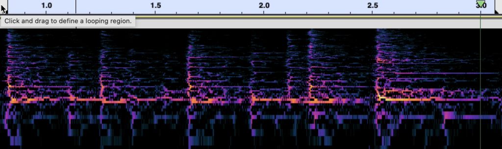
Media 2: Clifton James playing the “Bo Diddley rhythm” as a spectrogram.
James plays with a distinctive pattern of right-hand left-hand alternation along with alternation of stronger strokes to the centre of the tom and weaker strokes closer to the edges, which reflect the down and up strokes that Diddley will use when he plays the rhythm on guitar. The stronger strokes also vary in timbre depending on how much James allows the drum to ring, especially on the louder, more timbrally rich strike at the end of the measure. All these differences are visible to some extent in the spectrogram.
Musical notation is clearly limited in what it can show about the timbral and dynamic variations of different onsets, with accent markings and possibly other kinds of expressive indications doing what work they can. In the example, accents denote the stronger right-hand strokes, but other strokes also differ in how they are played. The idea of “the rhythm” abstracts away from some of these features but not all. Because the sounds of the drum are impulsive, this example at least permits us to maintain the fiction that a rhythm consists of a set of timepoints; that fiction would be more exposed by inquiring into the rhythm of the vocals, for instance. Nonetheless, it remains a fiction: even in a drumming pattern, the onsets of the pattern occupy finite timespans at some level. Also, we identify the Bo Diddley rhythm not only with this instantiation, but many repetitions of the rhythm by performers in many performances of this song and in others, and there clearly is some range of variation in precisely performed timing within the larger set of good representatives.
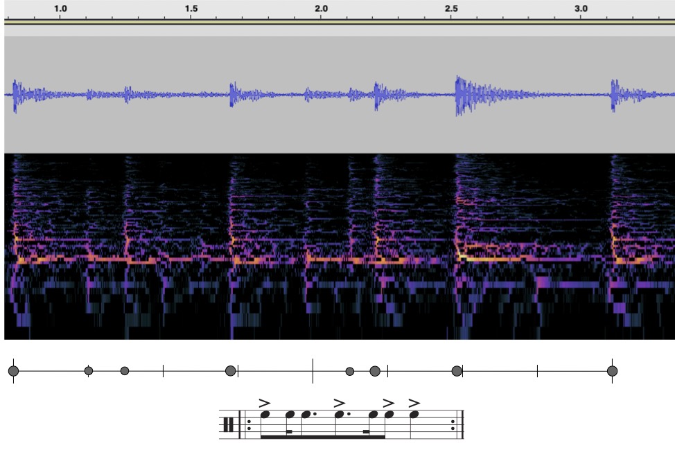
Figure 1: The Bo Diddley rhythm as a waveform, a spectrogram, points on a timeline, and notation.
Putting those matters aside for the moment, the musical notation in Figure 1 is inaccurate in its representation of the performed timing of the drum strokes, especially of the second, third, and fourth accented strokes of the pattern, which come earlier than the notation implies. One way to address this, when using notation as a descriptive tool, is simply to write the deviations as fractions of the beat duration under the notes that are played earlier than the notation implies. The method effectively factorizes the rhythm into the isochronous part representable in the notation and the deviations from that. Fernando Benadon (2024), many of whose arguments about the inadequacy of isochronous models of rhythm I echo here, uses a related approach of specifying non-integer proportions between successive timespans under otherwise temporally inaccurate notation. This idea of notation/microrhythm factorization is the basis of a large and productive research area within music psychology on expressive timing. Expressive timing is defined as deviation from the “metronomic” or “deadpan” timings theoretically implied by notation (Sloboda 1983; Bisesi and Windsor 2018). While this literature has been valuable for understanding performed rhythm, by requiring us to treat the metrical periodicities as absolute and fixed, it might be obscuring interactions of the precise timing with other periodicities.
Another possible strategy for representing timing deviations is to alter the notation to better approximate them, as in Figure 2. Although this kind of strategy is rarely if ever used in any serious way to study timing, it is revealing to ask why such an accommodation seems unrealistic. One could certainly make the argument that notation is able to approximate any desired rhythm to any desired finite level of accuracy. Notation like Figure 2 illustrates that such precision comes at a cost when the notation becomes overly complex. Perhaps what a musician will first notice about such notation is its unplayability. The purpose of the notational method of subdivision, after all, is prescriptive: it shows a player or singer how to count out the rhythm. At a certain point, the temporal divisions implied by the notation become too fast to count, and slowing down the tempo to learn a part can only accomplish so much. It is implausible prima facie that much of the information represented in Figure 2, such as the exact subdivisions used, could represent anything meaningful about Clifton James’s musical actions or a listener’s perception of them.
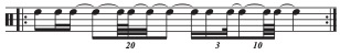
Figure 2: Alternate notation for the Bo Diddley rhythm, attempting to represent its timing more accurately in notation.
The notational complexity that that we perceive in Figure 2, the irrelevant information provided by the notation, is directly proportional to the level of precision that we demand of the notation. Notational complexity can be construed as the number of timepoints theoretically implied by the notation, ones that a musician would need to silently count to produce the rhythm in addition to those corresponding to actual onsets. This is a consequence, more abstractly, of the discrete time aspect of notation. “Discrete time” means that the notation posits a finite number of timepoints, which are by definition dimensionless, infinitesimal.1 Note that this remains true even though notation can include real-valued tempo indications. These could theoretically be used to account for timing deviations like those in Figure 1, but the timepoints designated by the notation remain discrete and infinitesimal, and a similar kind of impractical complexity results, with tempo changes potentially occurring multiple times within a beat to achieve a certain level of precision. This has consequences for adequately defining what it means for two such points to be close together or far apart in time, because discrete descriptions limit the ability to represent the space between them.
One prominent example of the limitations of a discrete, rational-number model of time is the study of swing ratios in jazz (Friberg and Sundström 2002; Benadon 2006, 2009, 2024; Honing and de Haas 2008). Musicians may sometimes explain swing using a rational-number model, for instance saying that the eighth notes of a swung rhythm have a triplet feel (a 2:1 ratio), or that a certain musician plays a dotted-eighth/sixteenth (3:1) swing instead of a triplet swing. This method quickly becomes useless when trying to express the fact that, for instance, the average swing ratio is between 1:1 and 2:1, or that swing ratios generally decrease as tempo increases. Although it is possible to notate a swing ratio, say, between 1:1 and 2:1 (e.g. using quintuplets), an increase in precision is only achievable through a corresponding increase in complexity. In practical terms, this results in unperformable (and therefore effectively irrelevant) notation for even modest degrees of precision. In theoretical terms, to do basic quantitative descriptions such as to average the swing ratio over a performance, or to define continuous functions such as one from tempo to average swing ratio, requires real numbers. Timing research therefore treats swing as a real-valued quantity, not a notatable rational quantity.
Usual conceptions of meter derive from the discrete model provided by musical notation. The idea of meter involves, most generally, a regularity or periodic occurrence of rhythmic events. However, the theoretically possible frequencies of events that might correspond to meter are strictly limited by the discrete-time basis of musical notation. The discrete-time problem of notation, that is, can be stated equivalently in terms of frequencies: notation lacks a continuum of metrical frequencies necessary to adequately define proximity relations between frequencies. This fact will become important in Section 4 below.
In observing problems with the notational fiction of instantaneous timepoints, I join other theorists who have pointed out the disconnect between this feature of notation and the real timing of musical performance. Authors such as Danielsen (2010) and Danielsen, Johansson, and Stover (2023) have proposed beat bins and related concepts for addressing this disconnect. I will propose a way of relating the concept of beat bins to the frequency-based approach of the next section through the Heisenberg uncertainty principle.
Simple periodic functions, frequency spaces, and spectra
These observations lead to the central proposal of this article: an approach based on simple periodic functions, which are continuous functions of time, as an alternative to the standard discrete-time theory of meter. These simple periodic functions are the basic elements of the Fourier transform, and in what follows in this section, I break down the process of the Fourier transform into its individual steps to help reveal the theoretical implications of each part. Although much of the virtue of using continuous functions to theorize rhythm and periodicity lies in extending to applications on timing measurements of performed music, my main focus will be to demonstrate that the continuous-time approach to periodicity is essential even when studying the quantized rhythms implied by notation.
Figure 3a shows one of the quantized versions of the Bo Diddley rhythm along with two simple periodic functions. The first is a cosine function and the second is a sine function, and both have a periodicity corresponding to the quarter-note beat. The cosine function tells us when notes are on the beat, with a value of 1, or halfway between beats, with a value of –1. The function continually oscillates between these two extremes, so that a note close to the beat will get a positive value, which is higher as the note gets closer. We can assess the total “on-beatness” of the rhythm by adding these values together. There is some information missing about the quarter-note periodicity of the rhythm, though, because a note ahead of the beat gets the same value as a note the same amount behind the beat. The sine function makes precisely these kinds of distinctions, with negative values preceding the beat and positive values following it. The two functions are oblique: the sine function hits zero where the cosine function has a maximum or minimum, and vice versa. Figure 3b does the same calculations for a different rhythm, the distinctive ostinato played by the guitar in another 1955 hit, Fats Domino’s “Ain’t That a Shame.”
Media 3: The distinctive ostinato played by the guitar in Fats Domino’s “Ain’t That a Shame” (1955). Listen to Media 3.
These two functions thus define a two-dimensional space, as shown on the right of Figure 3a and b, which takes the evaluation of the rhythm on the cosine function as a y value and the evaluation on the sine function as an x value.2 This is contrary to the usual mathematical convention which would plot the cosine value on the x-axis and the sine value on the y-axis. Putting the cosine on the y-axis produces the familiar music-theoretic “clockface” convention, with 0 pointing up. Every rhythm has a corresponding point in the space that gives essential information about how it expresses quarter-note periodicity. The angle of the point clockwise from the positive y-axis indicates where the balance of its weight falls in the quarter-note cycle. The distance from zero indicates how strongly it weights that spot. A rhythm in the upper part of the space is more on-beat, and in the lower part more off-beat. A rhythm on the left side of space has its weight more ahead of the beat, on the right side behind the beat. Circling the space one time corresponds to a continuous traversal of the quarter-note span. The Bo Diddley rhythm is at 180°, which means that its weight is on the off-beats, not favouring early or late, and it has the modest size of 1 because of its mix of on- and off-beat notes. Fats Domino’s rhythm, in contrast, gives a much larger vector, and one that points up, showing that it is strongly on beat. This is because the guitar plays on every beat and the distinctive triplet swing of the off-beat notes prevents them from fully cancelling out the on-beat notes. It also points to the left, because the off-beat notes are always ahead of the beat.
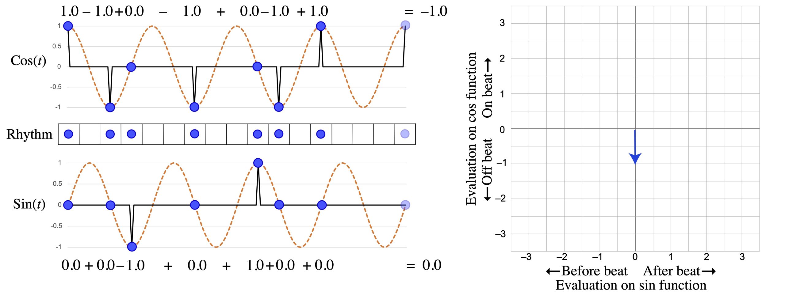
Figure 3a: Analysis of the Bo Diddley rhythm at the frequency of the quarter-note beat (f4).
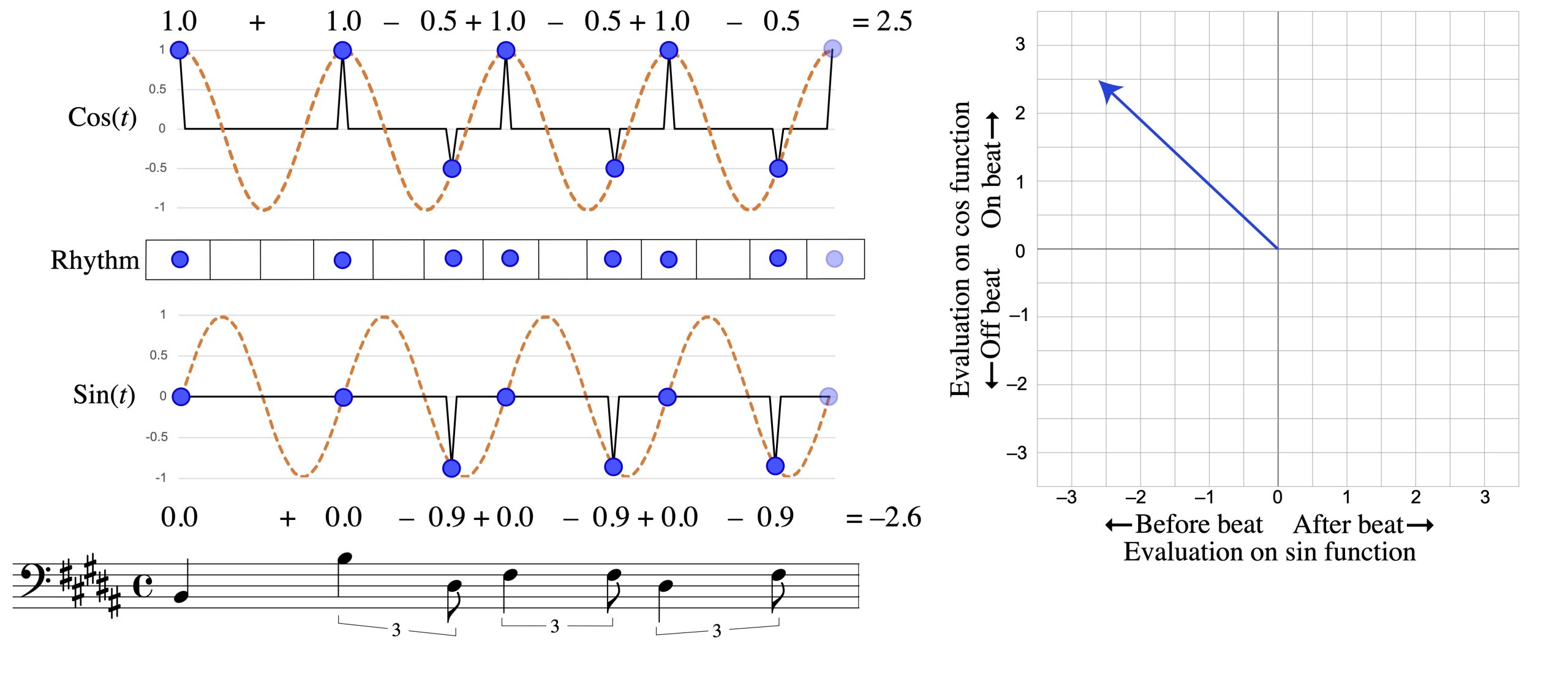
Figure 3b: Analysis of the “Ain’t That a Shame” guitar riff at the frequency of the quarter-note beat (f4).
We can use the same method to analyze other frequencies of a rhythm. For instance Figure 4a–b evaluate the Bo Diddley and “Ain’t That a Shame” rhythms on the half-note periodicity. Since the measure is a complete cycle, this is frequency 2 (1/2 measure), or f2, while the quarter-note periodicity is f4 (1/4 measure). Bo Diddley is equally balanced between on and off the half-note beats, but it is more behind the beat, as shown by the positive x value. The “Ain’t That a Shame” riff does not articulate the half-note periodicity as strongly as the quarter-note periodicity, because the notes on quarter-note beats totally balance out. The off-beat notes, however, tend to be closer to, and ahead of, beats 1 and 3, so the vector again points up and to the left.
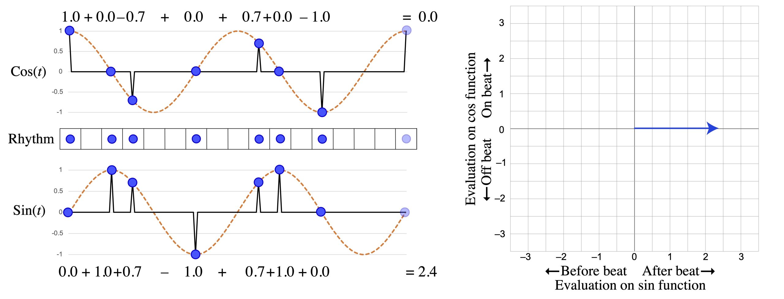
Figure 4a: f2 of the Bo Diddley rhythm.
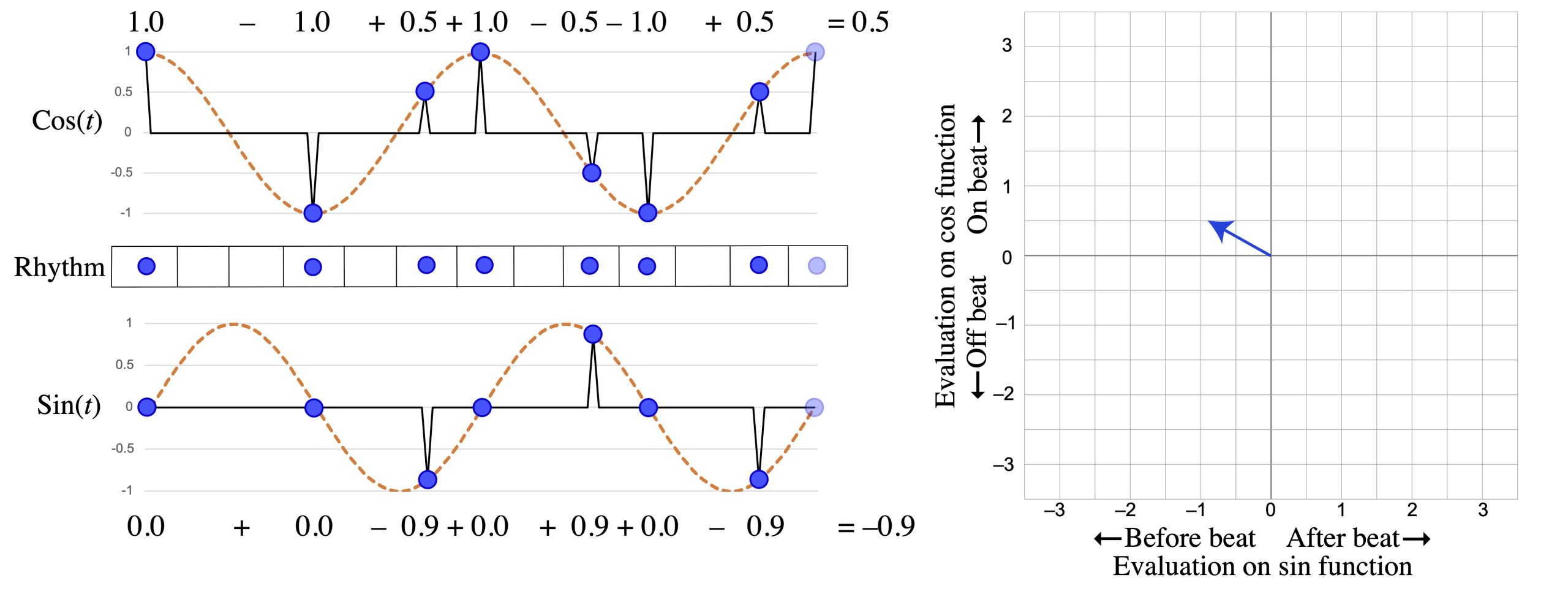
Figure 4b: f2 of the “Ain’t That a Shame” rhythm.
The two frequencies we have just considered relate to traditional metrical levels, and shows that the Bo Diddley rhythm (unlike the “Ain’t That a Shame” riff) does not articulate these very strongly. But the method is not limited to metrical periodicities. In Figure 5 the periodic function divides the measure by three. Only one of the peaks of such a function can be aligned with the eighth-note grid, but this is not a problem since the function is defined at every point in time. Onsets that positively weight the cosine function most strongly are those that are a dotted eighth-note away from the downbeat in either direction. The Bo Diddley rhythm also weights very weakly on f3.
In f3 the rhythm has a mixture of on-beat and after-beat qualities, so that its vector points at a 45º angle. This angle corresponds to a phase shift of the sinusoidal functions. By sliding the cosine function ahead by one-eighth of the f3 cycle as in Figure 5b, we can capture all the energy of the rhythm at this frequency in a single sinusoidal function.
Frequency 5, a division of the measure into 5 subcycles, also gives a vector at a 45º angle from the axes of the space, but this one is much larger than any of the others, as shown in Figure 6. This means the Bo Diddley rhythm has much more energy in this frequency than any of the others we have considered. This reflects a general fact, that a rhythm distributes its “energy” among the available frequencies, so a rhythm like the Bo Diddley that lacks metrical frequencies must have a prominent non-metrical periodicity. The phase shifted sinusoid shows the even division of the measure by 5 that the rhythm best approximates. Two peaks of this phase-shifted function line up with the third and fourth onsets of the rhythm, showing that these are central to the f5 quality of the rhythm.
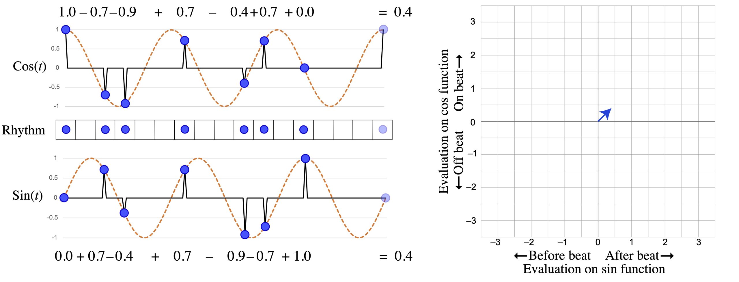
Figure 5: f3 of the Bo Diddley rhythm in two-dimensional f3 space (a) and as a single phase-shifted sinusoid (b).
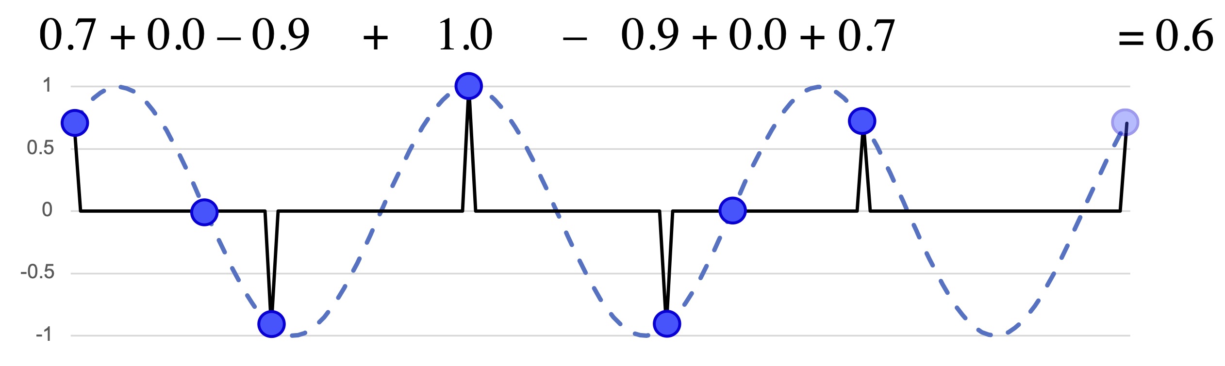
Figure 5b: f3 of the Bo Diddley rhythm as a single phase-shifted sinusoid.
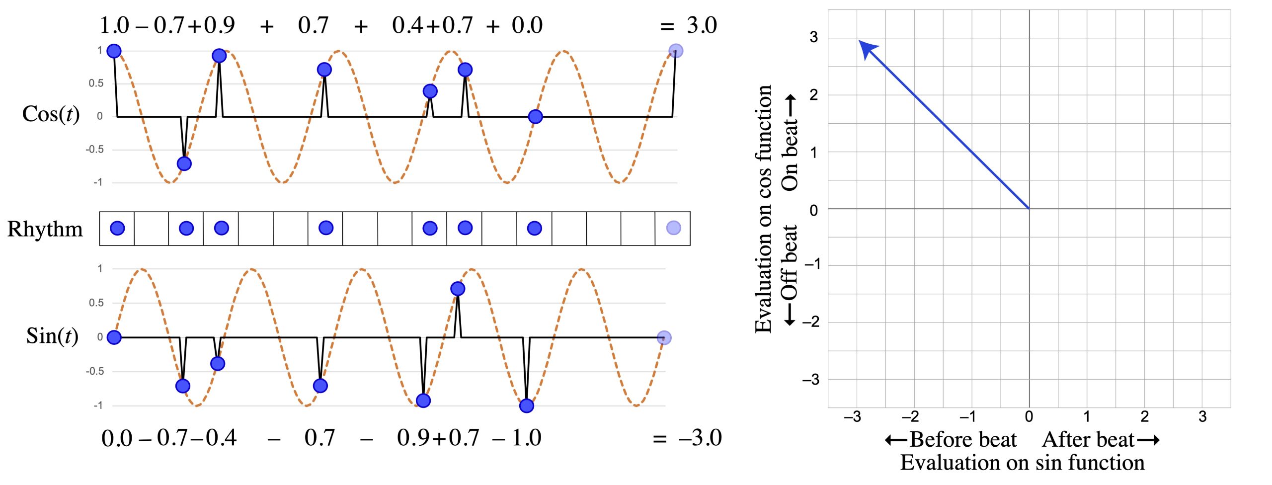
Figure 6a: f5 of the Bo Diddley rhythm in two-dimensional f5 space.
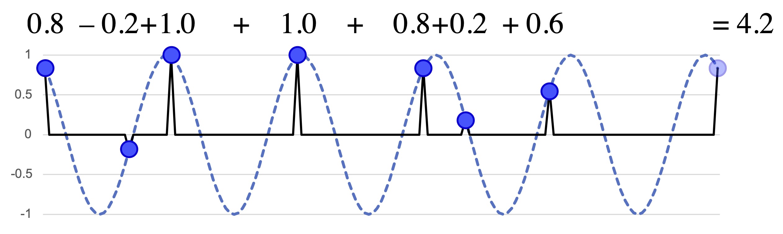
Figure 6b: f5 of the Bo Diddley rhythm as a single phase-shifted sinusoid (b).
The last two frequencies that we have considered, where the peaks do not line up with the eighth-note grid, do not correspond to anything in the traditional theory of meter. They may perhaps resemble the idea of a polyrhythm, but traditionally it only makes sense to speak of a polyrhythm when the onsets line up precisely with the conflicting divisions. One reason to pay attention to these off-grid frequencies is that they are part of the total information content of the rhythm. For a rhythm on a discrete grid of n timepoints per cycle, the frequencies from 1 to n/2 give a complete description.3 The calculations described here are the basis of the Fourier transform, which I use throughout this article. The assertion here is one of the fundamental Fourier theorems (invertibility). Many existing publications, such as Amiot 2016 and Yust 2021a–b, describe in detail the use of Fourier transform on rhythm. Another reason is that one of them might be the principal frequency component of some rhythm of interest, such as the Bo Diddley rhythm. As we have seen, this rhythm does not weight very heavily on any traditional metrical frequencies but does have a very strong f5. Off-grid frequencies are characteristic of rhythms associated with groove and clave or timeline rhythms.
One of the problems we initially encountered in defining the Bo Diddley rhythm was that certain aspects of the varying loudness and timbre of the onsets seemed to be essential features. The usual critical approach to the Bo Diddley rhythm is to equate it with the Cuban son clave rhythm, shown in Figure 7. There is some rationale to this claim, but it can also be misleading, because it misses some distinct features of the Bo Diddley rhythm, like the characteristic strumming pattern. There are four main accents in Bo Diddley’s rhythm, and they line up with four of the five notes of clave. Figure 7 plots these in the f5 space, along with two versions that apply the observed timing deviations from the beginning of the alternate studio take. All of these are relatively close together in the space, which reflects the fact that when using continuous functions to analyze a rhythm, small changes in the rhythm translate into relatively small displacements in the space. Therefore we can say that one of the characteristics of the Bo Diddley rhythm that remains stable over variations preserving the rhythm’s identity is a strong f5 in the upper left quadrant, centred on the second and third notes of the clave rhythm (meaning that peaks of the function at the bottom of Ex. 6 line up closely with these onsets). This explains why we might choose the clave rhythm as the best representative, since it has exactly one onset for each of the peaks of the f5 function. (For instance, in Diddley’s famous appearance on the Ed Sullivan Show in 1955, the audience claps along with “Bo Diddley” in a clave rhythm.) The second onset of the clave rhythm increases the size of f5 from the four emphasized notes while having no effect on the phase, so it makes sense to include it, since it only intensifies, without altering, the basic quality of the rhythm. On the other hand, the other unemphasized onsets have a similar effect to the timing deviations from isochrony, to move the rhythm further into the upbeat zone of the space.
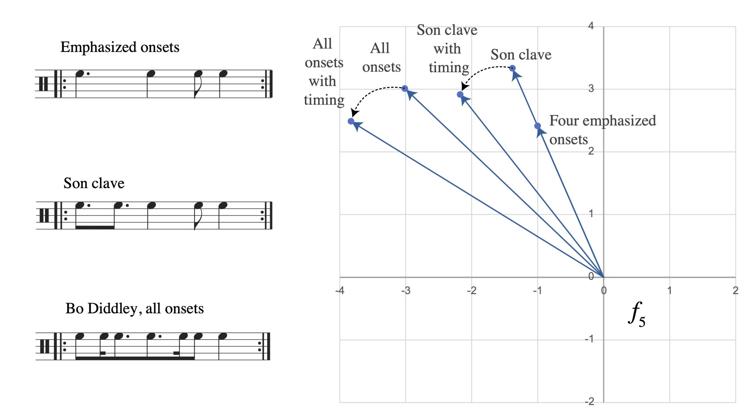
Figure 7: Variations on the Bo Diddley rhythm and their locations in f5 space.
Relatively small timing deviations like the ones in the Bo Diddley rhythm will necessarily have a small effect on relatively low frequencies like f4 or f5. To state this as a more precise rule, the deviations that we lose in quantizing to a grid of frequency n (here 16), will have limited effects on frequencies smaller than n/2 (8 in this case, the frequency of the eighth note). Therefore, one consequence of the theory proposed here is that the metrical significance of such distinctions of timing depends simply on how large a frequency range we consider to be relevant to “the meter.” In the previous section, I noted the affinity of the present approach to the beat bin idea of Danielsen (2010) and Danielsen, Johansson, and Stover (2023). Without going into too much detail, the obvious logical representation of the beat bin idea (though not proposed specifically by Danielsen herself) would be a Gaussian function, which can vary in width to model tighter or looser bins. A basic result of Fourier theory, the basis of Heisenberg’s uncertainty principle, is that a Gaussian function in time corresponds to another Gaussian function in frequency, with an inversely related width. As we tighten a beat bin in time, we expand it in frequency space. As we loosen temporal precision, we cut off higher frequencies. In other words, tightness of beat bins is mathematically equivalent to the span of relevant rhythmic frequencies, with higher frequencies becoming relevant as beat bins narrow.
Another important consequence of continuity of time, however, will primarily occupy the remainder of this article: even within a theory of meter limited to a relatively small frequency range (such as frequencies 1–8 here), the time-continuous model of periodicity can make smaller distinctions of frequency than a time-discrete one. The Bo Diddley rhythm, considering just the properties that it retains when restricted to a sixteenth-note grid (those observable in frequencies 1–8), strongly favours f5 over f4. With standard theories of meter, we can see the weak f4 (the rhythm is highly syncopated at the quarter-note level), but the strong f5 is only observable by switching to an implausibly complex representation (e.g. quantizing to a quintuplet-sixteenth grid).
To make these kinds of observations, comparing different frequencies, one additional representational tool will come in handy, the rhythmic spectrum. This shows only the magnitude of each frequency (the distance from zero), ignoring the phase (angle). Figure 8 gives spectra for all the Bo Diddley variations from Figure 7. The 4-onset rhythm is equally strongly described by a frequency of 3 as it is by a frequency of 5; however, as more notes are added to it f3 is suppressed and f5 enhanced. The microrhythmic variation has a relatively small effect, but when applied to the full rhythm it further increases f5 and decreases f3 by noticeable amounts. Applied to the clave rhythm alone it further weakens f4.4 The reader may also notice the increase in f2, which relates to the prominent bipartite division of clave rhythm that musicians often refer to as the “3-side” and “2-side” (Peñalosa 2012). This is enhanced by Bo Diddley’s added onsets.
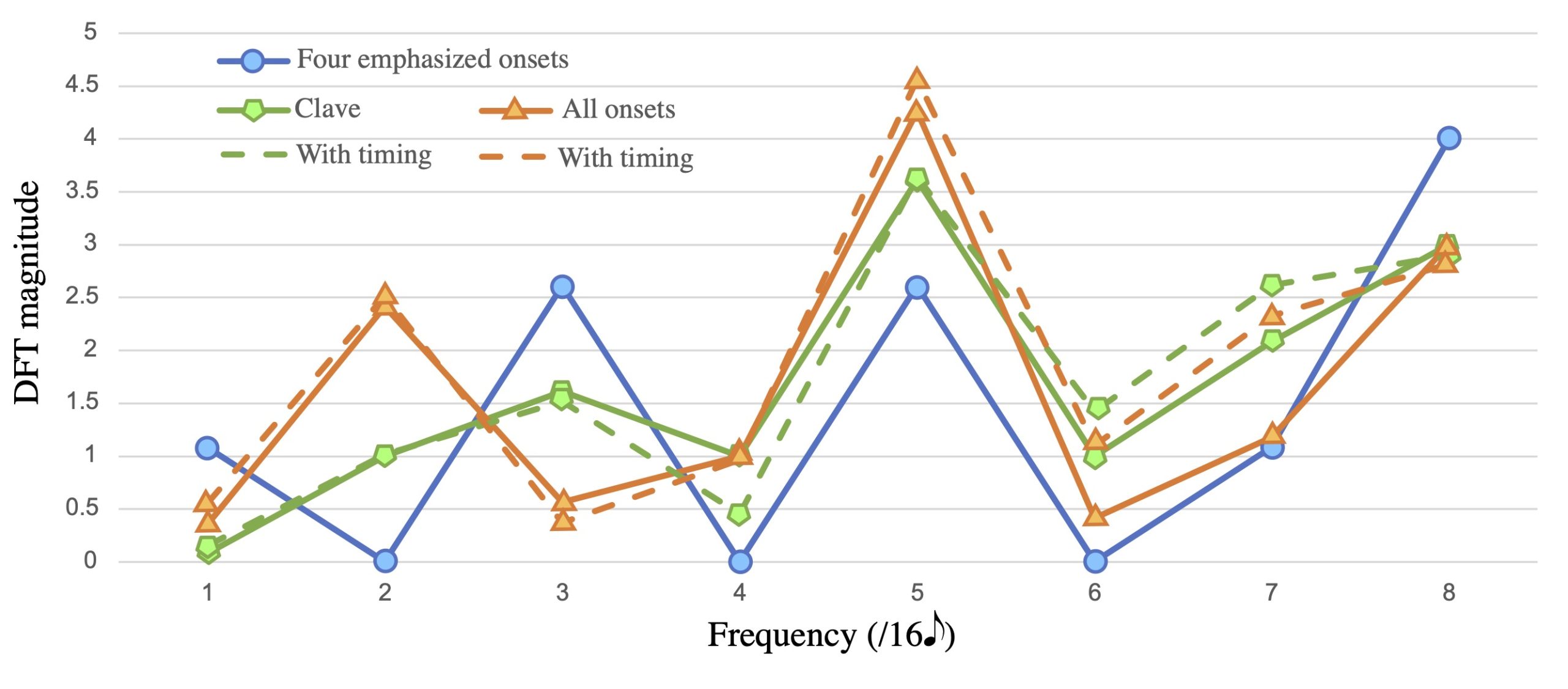
Figure 8: Spectra of different variations on the Bo Diddley rhythm.
Maximal Evenness
Many people have noticed the importance of maximally even rhythms in many different musical contexts (Pressing 1983; Rahn 1996; Toussaint 2013; Osbourne 2014). Often we find that maximally even rhythms play an important theoretical role beyond occurring frequently as literal rhythms, such as acting as a clave or timeline rhythm (Rahn 2021). For example, the tresillo and cinquillo rhythms, maximally even 3-in-8 and 5-in-8, are ubiquitous in Latin American music, ragtime, and other American popular music (Toussaint 2013; Cohn 2016), and the African “standard pattern” is maximally even 7-in-12.
The idea that the frequency components of a rhythm, as described in the last section, are important features explains why this might be the case. Maximally even rhythms are prototypes of the frequency corresponding to their cardinality, meaning they give a maximum possible value for their cardinality (Quinn 2006–2007; Amiot 2007, 2016). Therefore when a frequency does not correspond to a simple metrical division of the cycle, relating a rhythm to a nearby maximally even one is a way of understanding how it expresses that frequency.
We can generalize this observation to generated rhythms, meaning ones that can be derived by iteration of a single interval. To see why this is the case suppose we are interested in rhythms that express a certain frequency as strongly as possible, but we are also limited to some isochronous grid. If the size of the rhythm does not evenly divide the frequency, then it is not possible to align the onsets precisely at the peaks of the curve. For instance Figure 9 shows a frequency of 5 over a sixteen-unit grid. The best we can do is find the multiple of a sixteenth note that gives the best approximation to some multiple of the periodicity. Three sixteenth notes is close to a fifth of the measure. We can add notes at intervals of 3 sixteenth notes above and below 0 to get the highest values possible on the function, resulting in a generated rhythm. As we add more notes the onsets get further away from the peaks.
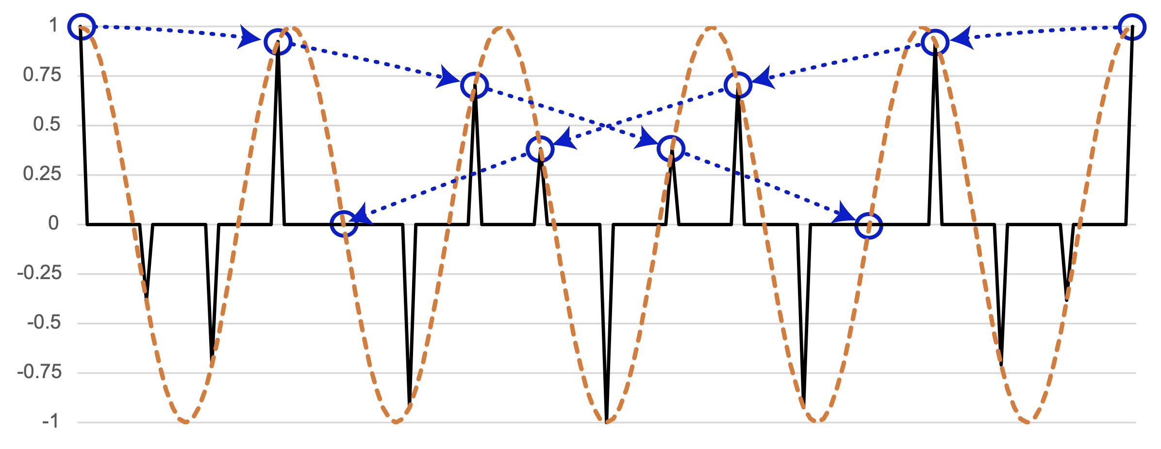
Figure 9: Maximizing a frequency through approximation, resulting in a generated rhythm.
The son clave rhythm discussed in the previous section is a good example of a rhythm that strongly expresses one non-metrical frequency (f5) but is not maximally even. Peñalosa (2012) shows how this rhythm belongs to a family of clave rhythms used in Cuban music, starting with a common African timeline rhythm, shown in Figure 10. This rhythm is 5-in-12 maximally even, the complement of the “standard pattern,” and interchangeable with it in many contexts. It and its rhumba clave variant also appear in many folkloric styles of Cuban music (Peñalosa 2012). Figure 10 shows their spectra extending up to 11, illustrating a mirror symmetry around n/2 that characterizes the spectrum of any n-gridded rhythm. According to this mirror symmetry, the magnitudes of f5 and f7 are constrained by the grid to be the same.
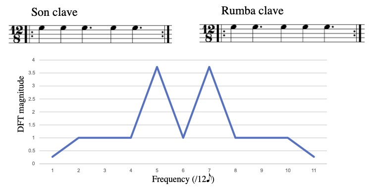
Figure 10: Two 5-in-12 maximally even clave rhythms and their spectrum.
The son clave rhythm is an approximation of this 5-in-12 maximally even rhythm on a grid of 16xs. One can derive it by matching the rhythm on the beats and squeezing the second and third positions of each triplet division of the 12/8 beat into the third and fourth sixteenth of every division of the 4/4 beat, as Figure 11 shows.5 See Peñalosa 2012. Interestingly, this timeline, originating as a Cuban modification of an African timeline, returned to West Africa via American R&B music to become the bell pattern for the Kpanlogo dance of Ghana in the 1960s (Collins 1992, p. 44; Ladzekpo 1996). Musical contexts that mix the two metrical feels (12/8 and 4/4), can feature continuous variation of off-beat notes between these positions (Stover forthcoming). The same transformation applied to the 12/8 rumba clave gives a 4/4 rumba clave which is not rotationally equivalent to the 4/4 son clave.
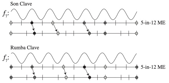
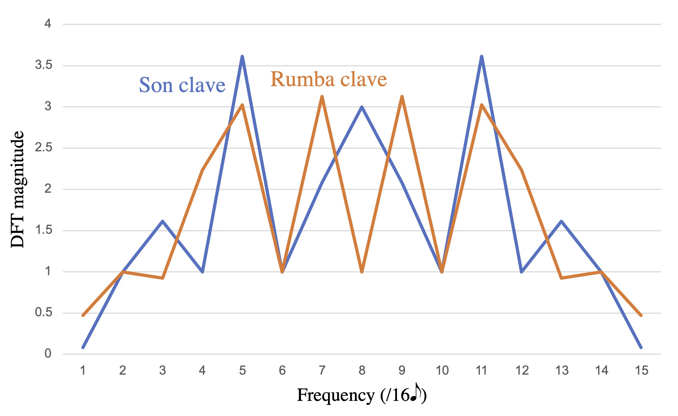
Figure 11: Derivations of 4/4 son clave and rhumba clave and their spectra – the shading of the dots indicates their centrality to the f7 function shown.
We can understand the effect of these displacements on the f5 and f7 frequencies of the rhythms by considering where the mobile notes occur with respect to the periodic functions. Moving notes central to the function, near a peak, will affect the phase of the function more and the magnitude less, whereas moving more peripheral notes will affect the magnitude more. Because the 12/8 clave rhythms are 5-in-12 ME, all the notes are relatively central to f5, and therefore f5 remains large in both 4/4 claves. However, the displacements of notes are larger relative to the narrower cycles of f7. The son clave differs from the rumba clave in that one of the larger displacements occurs on a peripheral note (the third onset), and the displacement is away from the peak, resulting in a marked decrease in the magnitude of f7. The “energy” of the rhythm, however, is constant,6 More precisely, the power of the rhythm is the sum of the squared magnitudes of the frequency components, and a fixed cardinality rhythm with all notes equally weighted has a constant power. so the magnitude that f7 loses must go somewhere, and the spectra show where: into a nearby frequency, f8, the eighth-note frequency. In other words, the primary difference between the 4/4 son clave and rumba clave is that in the former case, the displacement from maximal evenness shifts energy from f7 to the neighbouring f8, resulting in a rhythm that weights heavily on the eighth-note grid. By contrast, the rumba clave retains a strong f7 and could be described as a subset of a 7-in-16 maximally even rhythm.7More specifically, it is second-order maximally even, 5-in-7-in-16. See Douthett and Clough (1991).
Interaction of frequencies
The first part of this article argued for modeling rhythmic periodicity with continuous functions because they are able to reflect temporal proximity. The importance of temporal proximity for analyzing timing is self-evident, but much of the discussion above has dealt with rhythms as represented in notation, restricted to a discrete grid. Nonetheless, the use of continuous functions has made it possible to analyze rhythms as representatives of frequencies that do not evenly divide the timepoint grid. We also noted that, because they derive from continuous functions, frequencies also relate by proximity. One example in the last section, relating different clave rhythms, indicated the possible significance of proximity between frequencies. This section considers the implications of frequency proximity more generally.
The previous section mentioned the African standard pattern as an important rhythm that is maximally even and a prototype of a frequency that does not divide its temporal grid evenly. The musical significance of this frequency is, at least in part, its proximity to two metrical frequencies, f4 and f6. In West African drum ensembles that use the standard pattern or related high-f5 patterns, the beat corresponds to f4 while f6 is an important cross rhythm, what Ladzekpo (1995) calls the “secondary beat scheme.” Figure 12 shows how Ladzekpo derives the standard pattern from an alternation of two halves of two 6-against-4 polyrhythms. The alternation of on- and off-beat 6-beat schemes reflects a slow phase shift between the f5 periodicity underlying the standard pattern and the f6 periodicity of the secondary beat scheme illustrated at the bottom of Figure 12.
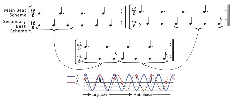
Figure 12: Ladzekpo’s (1995) construction of the standard pattern from two 6-against-4 polyrhythms, and the equivalent understood as a slow phase shift between a 7-in-12 maximally even rhythm (standard pattern) and an isochronous rhythm of 6 beats per measure (secondary beat scheme).
Ladzekpo describes the aesthetic effect of this kind of cycling of in-phase and out-of-phase with reference to the 3-against-2 polyrhythm that results from the combination of the 4-beat and 6-beat schemes:
Discovering the character of a cross rhythm simply implies absorbing the distinct texture produced by the interplay of the beat schemes, noting the distinct rate of speed with which they coincide or disagree. When the beat schemes coincide, a static effect (standing still) is produced and when they are in alternate motions an effect of vitality (fast-moving) is produced. […]
In aesthetic expression, a moment of resolution or peace occurs when the beat schemes coincide and a moment of conflict occurs when the beat schemes are in alternate motion. These moments are customarily conceived and expressed as physical phenomena familiar to a human being. A moment of resolution is expressed as a human being standing firm or exerting force by reason of weight alone without motion while moment of conflict is expressed as a human being travelling forward alternating the legs. (Ladzekpo 1995)
The same kind of slow phase shift results from the interaction of the f5 of the timeline with the f4 of the beat, as shown in Figure 13.
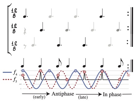
Figure 13: Slow phase shift between a 7-in-12 maximally even rhythm (standard pattern) and 4 isochronous beats (primary beat scheme).
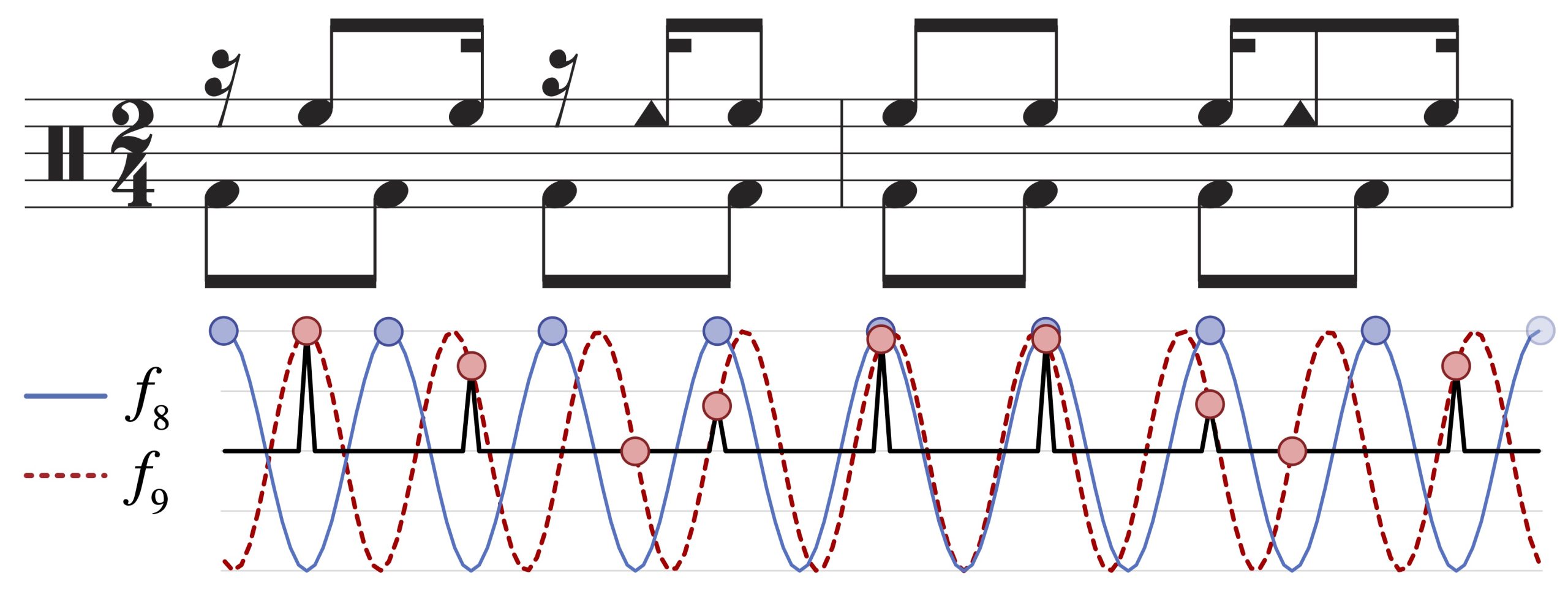
Figure 14: A samba timeline and its slow phase-shift relation to the isochronous eighth-note layer of the meter.
These sorts of slow phase shift patterns result when any two frequencies differ by a small amount. They have been recognized as a property of strict polyrhythms, for instance in the convergence-divergence patterns that Link (1994) identifies as a means by which Elliott Carter derives formal structures from long range polyrhythms. The principle is mathematically equivalent to combination tones or acoustical beats in the pitch domain, where the frequency of the slow phase shift is equal to the difference between the two interacting frequencies. For example, the 5-against-6 and 4-against-5 patterns go in and out of phase with a frequency of 6 – 5 = 5 – 4 = 1—i.e., one cycle per measure. On the other hand, the basic 6-against-4 polyrhythm that Ladzekpo refers to in the quote above has a frequency difference of 6 – 4 = 2, meaning that the parts cycle in and out of phase twice per measure.
György Ligeti, who experimented with complex polyrhythm in his later works (such as his sixth and twelfth piano études), also exploited this kind of phasing between rhythms with prominent non-metrical frequency components. His eighth piano étude, “Fém,” is based on two rhythms in counterpoint that repeat at different rates: 18e in the right hand and 16e in the left hand.8 The following analysis expands upon one from Yust 2017. The rhythms and their spectra are given in Figure 15, with the spectra scaled to align equivalent frequencies (since the frequency numbers for the left hand refer to divisions of a 16e cycle and the right-hand frequency numbers divide an 18e cycle). The largest (highest magnitude) components of the left-hand rhythm are f8, f4, and f7, while the largest components of the right-hand rhythm are f5 and f8. The frequency difference between f4 in the left hand and f5 in the right hand is 5/18 – 4/16 = 1/36, which means that these two frequency components go in and out of phase once every 36e, or 3 measures of 12/8. The smaller peak in the right hand at f8 is even closer to f7 in the left hand, at 8/18 – 7/16 = 1/144. Figure 16 shows how these create long patterns of the rhythms going in and out of phase. It helps to separate the two processes by splitting each rhythm into the onsets more central to the lower frequencies (f4/16 and f5/18) and the higher frequencies (f7/16 and f8/18). This is shown with colour coding in Figure 16, where the part of each rhythm primarily expressing the lower frequency is in blue and the part primarily expressing the higher frequency is in red. Similar local patterns between the right-hand and left-hand subrhythms represent the proximity of their characteristic frequencies.
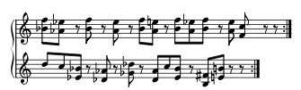
Figure 15a: The two repeating rhythms from Ligeti’s “Fém”.
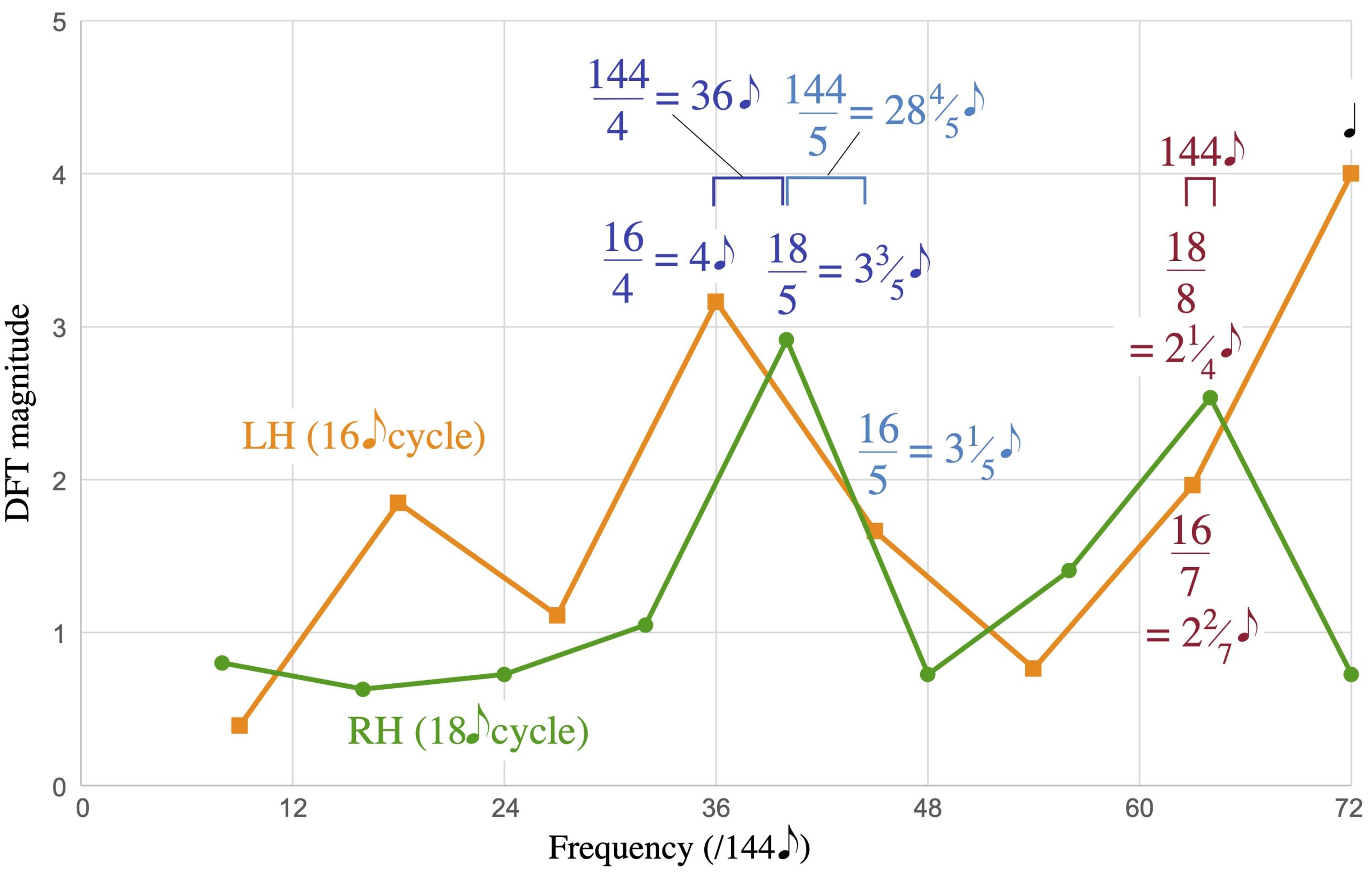
Figure 15b: The spectra of the repeating rhythms in Ligeti’s “Fém” – spectral peaks and differences are labelled with their periodicities.
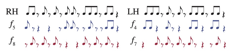

Figure 16: The two ostinato rhythms from “Fém,” split into subrhythms made up of onsets most central to f4/16 and f5/18 (blue and purple) and f7/16 and f8/18 (red and purple), and a full cycle of the combined ostinati with curves showing the cycles of coincidence and interlocking created by the interactions of f4/16 and f5/18 (blue), f7/16 and f8/18 (red), and f5/16 and f5/18 (light blue).
On one level, the illustration in Figure 16 helps to explain the overall pattern of reinforcement and interlocking, which is quite salient. The 36e periodicity (frequency 4/144e) stands out especially at this level, leading to many coinciding attacks in mm. 3, 6, 9, and 12, and interlocking patterns in mm. 2, 5, and 11. Another way to read Figure 16 is to note that where the periodicities of interaction disagree, the overall rhythm of coinciding attacks is dominated by the quality of whichever periodicity is positive at that point. For the 36e periodicity that is a eeä ä eeä ä rhythm and for the 144e periodicity it is a eä eä eä rhythm. The point of maximum agreement between all three functions is at the end of the 144e cycle where the long rest lines up in the two parts, which Ligeti uses to signal the completion of a cycle.
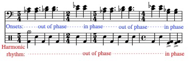
A similar example appears in the first movement of Ligeti’s Piano Concerto, a pivotal work (Steinitz 2011). The method here is somewhat more complex because the two repeating rhythms, shown in Figure 17, involve a difference of subdivision (triplet eighths vs. duplet eighths) as well as a difference in cycle length (10q in the percussion/piano part and 12q in the strings). The resulting 15-measure cycle is shown in Figure 18. As the spectra in Figure 17 show, the three main peaks of the strings rhythm nearly coincide with three of the four largest components of the piano/percussion rhythm, all being at a frequency distance of 1/(60q), corresponding to a full cycle (60q = 15 mm.) periodicity. In addition, distances of 1/(12q) between the larger values in the spectra of Figure 17 create a noticeable convergence pattern in 3-measure cycles. Because of the different subdivisions, the slow process of phasing involves not only prominent coinciding attacks, e.g. in m. 3, but also gradual transitions through near-coinciding attacks, as in mm. 4–7 and mm. 12–15, to interlocking patterns, as in mm. 8–11, where the attacks in one part evenly divide the spans between attacks in the other.
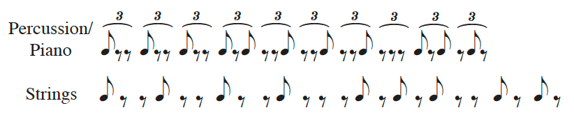
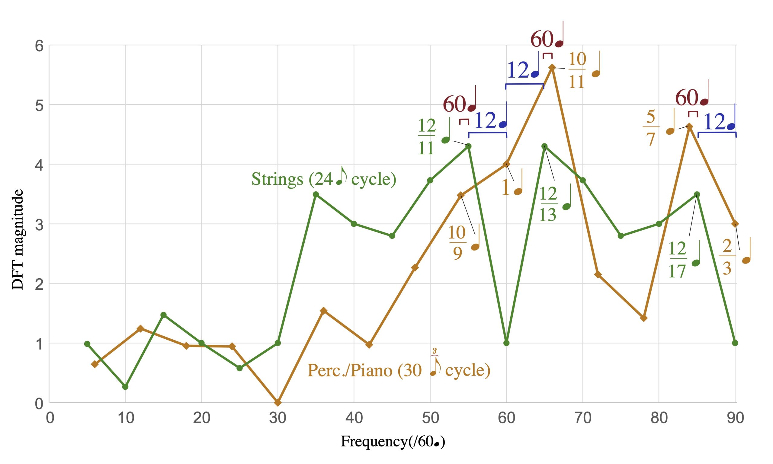
Figure 17: The ostinati from Ligeti’s Piano Concerto, first movement, and their spectra, with large values and frequency differences between large values labeled by their periodicities.
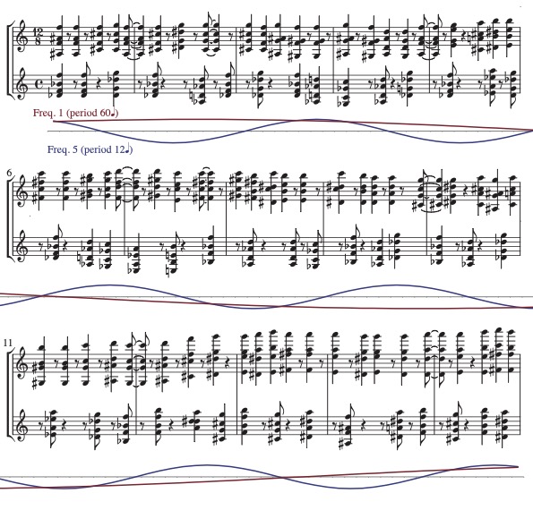
Figure 18: A reduced score of mm. 1–15 of Ligeti’s Piano Concerto, first movement, showing only the octave attacks in the piano and the string pizzicato chords – functions below the staff show periodic coincidence-divergence cycles.
We find similar techniques in works of contemporary jazz composers known for their rhythmic experimentation. A relatively straightforward example can be found in the B part of “You Can’t Say Poem in Concrete” by the Dave King Trucking Company, shown in Figure 19. The quarter notes of the rock-style backbeat pattern in the drums (frequency 16/32) interact with the surface rhythm of the guitar peaks at f14/32 to give a phasing cycle of 8q, half of the full 16q cycle (frequency 16/32 – 14/32 = 2/32). By a similar mechanism, the harmonic rhythm of the guitar phase-shifts with the half-note beat over the full 16q cycle.
Media 4: Audio example of the Ostinati of the B and C parts of “You Can’t Say Poem in Concrete” by the Dave King Trucking Company. Listen to Media 4.
![]()
Figure 19: Ostinati of the B and C parts of “You Can’t Say Poem in Concrete” by the Dave King Trucking Company, and spectra.
The C section of “You Can’t Say Poem in Concrete” is based on a repeating melody in 13/8 which, like the guitar part in section B, is close to maximally even rhythm. Because of the similarity to maximally even rhythms, both parts have one prominent peak, and these are associated with very similar periodicities, which we can derive by inverting the frequency numbers, 32/14 = 2 2/7e and 13/5 = 2 2/5e. When we consider the slight increase in tempo from about e = 230 to e = 236, these periodicities are even closer (from about 101 BPM to 91 BPM). This creates a continuity between the sections that otherwise contrast rhythmically in fundamental ways, from a long (32e) cycle to a short (13e) cycle and from a relatively sparse rhythm of quarters and dotted quarters to a faster rhythm in mostly eighths and quarters.
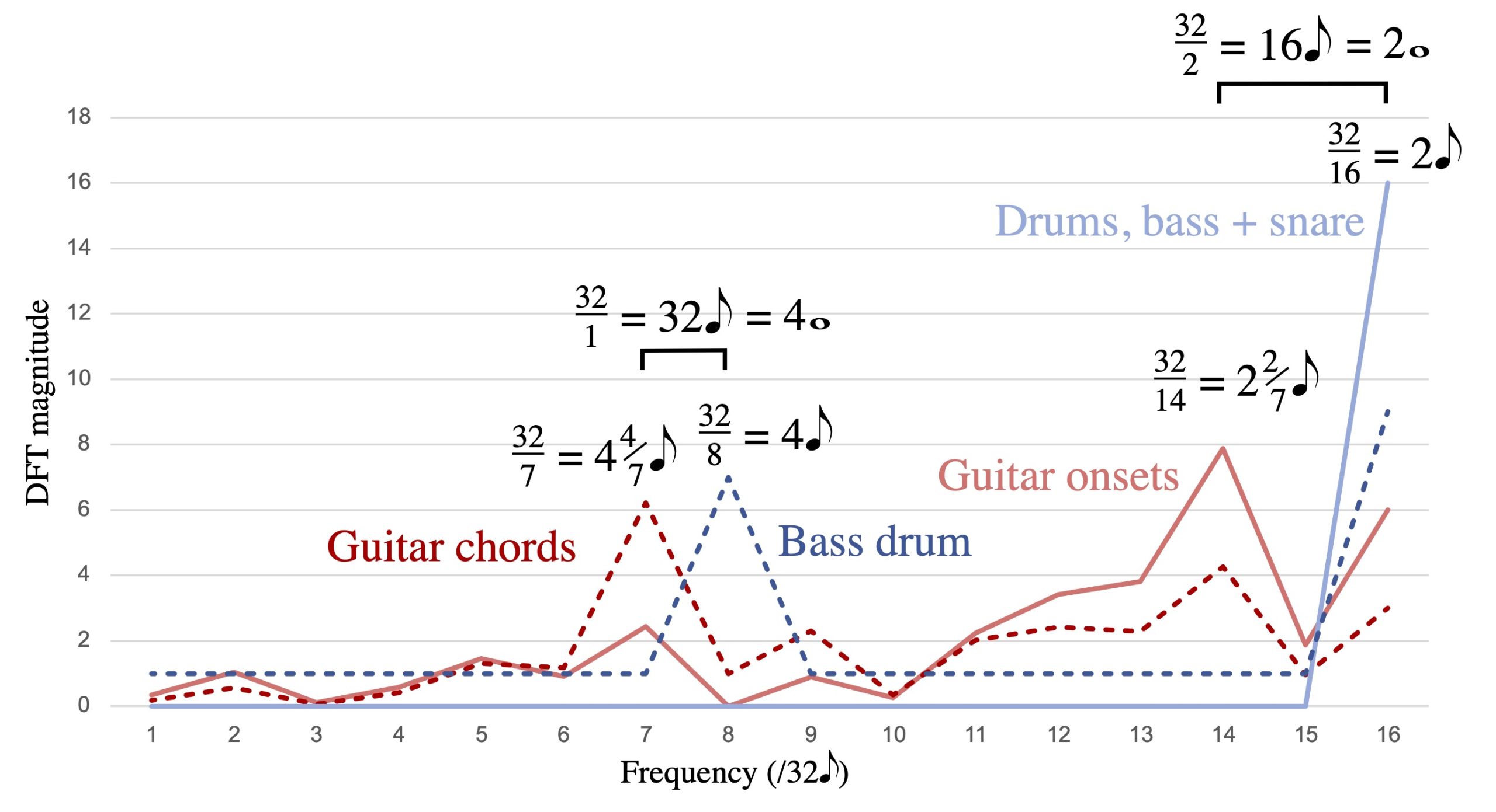
Guitarist Miles Okazaki takes advantage of similar kinds of interactions between ostinato patterns in his compositions. Figures 20–22 show ostinati that make up the accompanying parts for “Eating Earth,” written for his Trickster quartet. A way to simplify these is to regularize the bass part by ignoring the single 1e correction at the beginning that Okazaki uses to fit 9 repetitions of the 7e pattern into 8 measures of 4/4. The resulting interaction between f3/5 and f4/7 gives a phasing cycle of 35e, shown in Figure 21. Okazaki’s music is full of relatively simple maximally even patterns like this that repeat at odd rates, combined within a duple metrical framework, so that the phasing of the patterns both with the metrical context and with one another are salient. He has also developed methods of rhythm training where practising of these kinds of patterns is central (Okazaki 2015, 2016).
Media 5: Audio example of the ostinati that make up the accompanying parts for Miles Okazaki’s “Eating Earth,” written for his Trickster quartet. Listen to Media 5.
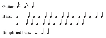
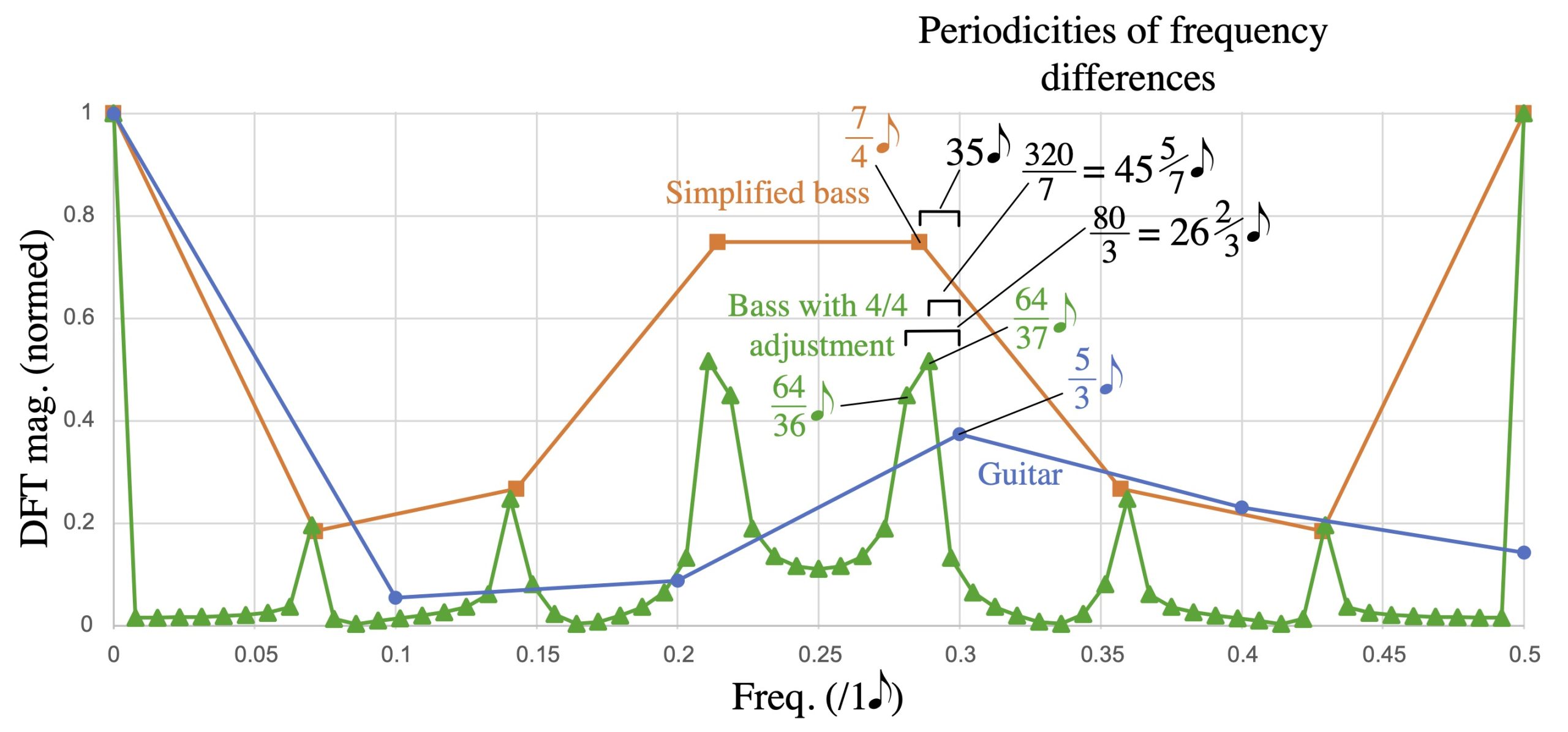
Figure 20: Ostinati for the bass and guitar for Miles Okazaki’s “Eating Earth” (Trickster, 2017), and their cardinality-normalized spectra, treating the bass part both as a simple 7e-cycle rhythm (ignoring the 1e correction) and as a complete 64e-cycle rhythm.
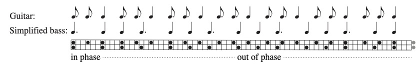
Figure 21: Guitar ostinato combined with a simplified version of the bass ostinato, creating a 35e phase-shifting cycle.
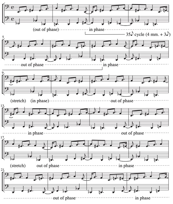
Figure 22: The first 24 measures of ostinati realized in score form. The guitar part is simplified to onsets where the pitch changes. (The surface rhythm is the complement of this, so it has the same spectrum.) Annotations below the staff show the 35e phasing cycles of the 7e simplified bass pattern and the 5e guitar pattern.
If we analyze the rhythm including the hiccup that results from the 1e correction in the bass part, we get the “with adjustment” spectrum in Figure 20. It is a 64e pattern that approximates an oversampled version of the 7e pattern. The relevant peak now has a spread, which can be understood as an ambiguity about whether the five 1e hiccups stretch the 35e cycles when they occur or truncate them, as shown in Figure 22. According to the stretching interpretation, for instance, there are 2 cycles from the in-phase point in m. 3 to the in-phase point in m. 13, over a little more than 10 measures, representing the frequency of 7/320, 7 convergence cycles over the full 40-measure grand cycle. If, instead, we see mm. 7–9 as a separate truncated cycle, we get 3 cycles over about 10 measures, representing the frequency 3/80, which results in 12 convergence cycles over the full 40-measure grand cycle (one more cycle for each of the five hiccups).
This last analysis illustrates multiple ways in which frequency proximity is significant, and also relates to the point about Heisenberg uncertainty above. As in all the analyses in this section (Exx. 12–19), the length of a phasing pattern between ostinati depends on proximity of frequencies, with longer phasing patterns resulting from smaller frequency differences. However, in this case there are three possible ways to interpret the bass ostinato, resulting in three possible ways to measure the length of the phasing pattern ranging from around 3–6 measures. Proximity between frequencies also determines these three possibilities: when Okazaki accommodates the 7e pattern to fit into a 64e cycle, the energy of the spectral peak for the 7e pattern goes into the two nearest frequencies dividing the 64e cycle. Musically, however, the distinctions between these interpretations makes little, perhaps even negligible, difference. This is where the Heisenberg uncertainty principle is helpful. It tells us that there is a reciprocal relationship between temporal precision and frequency precision. Distinguishing very close frequencies of 0.281, 0.286, and 0.289 in Figure 20 requires a very wide temporal window of multiple measures. To the extent that our musical experience of these interacting rhythms is more localized, the differences between these frequencies is immaterial. When I invoked the Heisenberg uncertainty principle earlier, it was to explain how making small temporal distinctions (microrhythm) requires wide frequency windows; here we see the inverse, how small frequency distinctions require wide temporal windows.
Conclusion
I have only scratched the surface here of the possibilities of a rhythmic theory based on simple periodic functions. The tools of frequency spaces and spectra come from the Fourier transform, whose application to rhythm has been explored elsewhere, along with some of the more mathematical considerations largely sidestepped here (Amiot 2016; Milne, Bulger, and Herff 2017; Yust 2021a, b; Chiu and Yust 2022). Although the basic objects of my approach here, frequencies, might seem new, on some level they are as old as music itself, the same general concept that gives us the beating hand of the conductor and the measures, beats, and subdivisions of musical notation. The difference I have highlighted here is that frequencies (or, inversely, periodicities) in musical notation are discrete isochronous timepoint sequences, in contrast with the beating hand of a conductor or the sympathetic resonances of the metrically entrained brain, which, like the simple periodic functions of the theory presented above, are continuous and oscillatory. While traditional, discrete-timepoint–based metrical theory prioritizes hierarchically nesting timepoint sequences, problematizing polymeter, an approach based on continuous periodic functions provides tools for relating all kinds of rhythmic frequencies and can identify non-nesting frequencies in rhythms without the precise timing distinctions needed to articulate complex polyrhythms. These include the proximity relations discussed in part 4. Similarly, the continuous-periodicity approach can handle microtiming without the unbounded increases in complexity that burden representations in traditional music notation.
Bibliography
Agawu, Kofi (2003), Representing African Music. Postcolonial Notes, Queries, Positions, New York, Routledge.
——— (2016), The African Imagination in Music, New York, Oxford University Press.
Allgayer-Kaufmann, Regine, (2010), “From the Innocent to the Exploring Eye. Transcription on the Defensive,” The World of Music, vol. 52, no 1/3, pp. 416–431.
Amiot, Emmanuel (2007), “David Lewin and Maximally Even Sets,” Journal of Mathematics and Music, vol. 3, no 2, pp. 157–72.
——— (2016), Music Through Fourier Space. Discrete Fourier Transform in Music Theory, Heidelberg, Springer.
Benadon, Fernando (2006), “Slicing the Beat. Jazz Eighth-Notes as Expressive Microrhythm,” Ethnomusicology, vol. 50, no 1, pp. 73–98.
——— (2009), “Time Warps in Early Jazz,” Music Theory Spectrum, vol. 31, no 1, pp. 1–25.
——— (2024), Swinglines. Rhythm, Timing & Polymeter in Musical Phrasing, Oxford University Press.
Bisesi, Erica and W. Luke Windsor (2018), “Expression and Communication of Structure in Music Performance. Measurements and Models,” in Susan Hallam, Ian Cross, and Michael H. Thaut (eds.), The Oxford Handbook of Music Psychology, New York, Oxford University Press, pp. 615–631.
Butterfield, Matthew (2010), “Participatory Discrepancies and the Perception of Beats in Jazz,” Music Perception vol. 27, no 3, pp. 157–76.
Caplin, William (1981), “Theories of Harmonic-Metric Relationships from Rameau to Riemann,” PhD diss., University of Chicago.
Chiu, Matthew, and Jason Yust (2022), “Identifying Metric Types with Optimized DFT and Autocorrelation Models,” in Mariana Montiel, Octavio A. Agustín-Aquino, Francisco Gómez, Jeremy Kastine, Emilio Lluis-Puebla, and Brent Milam (eds.), Mathematics and Computation in Music, 8th International Conference MCM2022, Cham, Springer, pp. 343–348.
Clayton, Martin (2008), Time in Indian Music. Rhythm, Metre, and Form in North Indian Rag Performance, New York, Oxford University Press.
——— (2020), “Theory and Practice of Long-Form Non-Isochronous Meters. The Case of the North Indian rūpak tāl,” Music Theory Online, vol. 26, no 1, https://mtosmt.org/issues/mto.20.26.1/mto.20.26.1.clayton.html
Clough, John, and Jack Douthett (1991), “Maximally Even Sets,” Journal of Music Theory vol. 35, no 1/2, pp. 93–173.
Cohn, Richard (2016), “A Platonic Model of Funky Rhythms,” Music Theory Online vol. 22, no 2, https://mtosmt.org/issues/mto.16.22.2/mto.16.22.2.cohn.html
Collins, John (1992), West African Pop Roots, Philadelphia, Temple University Press.
Costa-Faidella, Jordi, Elyse S. Sussman, and Calres Escera (2017), “Selective Entrainment of Brain Oscillations Drives Auditory Perceptual Organization,” NeuroImage, vol. 159, pp. 195–206.
Danielsen, Anne (2010), “Here, There and Everywhere: Three Accounts of Pulse in D’Angelo’s ‘Left and Right’,” in Anne Danielsen (ed.), Musical Rhythm in the Age of Digital Reproduction, London, Taylor & Francis, pp. 19–35.
Danielsen, Anne, Mats Johansson, and Chris Stover (2023), “Bins, Spans, and Tolerance. Three Theories of Microtiming Behavior,” Music Theory Spectrum, vol. 45, no 2, pp. 181–198.
Friberg, Anders, and Andreas Sundström (2002), “Swing Ratios and Ensemble Timing in Jazz Performance. Evidence for a Common Rhythmic Pattern,” Music Perception, vol. 19, no 3, pp. 333–349.
Gotham, Mark (2015), “Meter Metrics. Characterizing Relationships Among (Mixed) Metrical Structures,” Music Theory Online, vol. 2, no 2, https://mtlosmt.org/issues/mto.15.21.2/mto.15.21.2.gotham.php
Honing, Henkjan and W. Bas de Haas (2008), “Swing Once More. Relating Timing and Tempo in Expert Jazz Drumming,” Music Perception, vol. 25, no 5, pp. 471–476.
Iyer, Vijay (2002), “Embodied Mind, Situated Cognition, and Expressive Microtiming in African-American Music,” Music Perception, vol. 19, no 3, pp. 387–414.
James, Clifton and Fish, Scott K. (2015), “I Wanted my Own Style of Playing”(interview), in Scott K. Fish, Life Beyond the Cymbals, https://scottkfish.com/2015/12/09/clifton-james-i-wanted-my-own-style-of-playing/
Ladzekpo, C.K. (1995), Foundation Course in African Dance Drumming, self-published, available at https://www.richardhodges.com/ladzekpo/Foundation.html
——— (1996), Kpanlogo Song Book, self-published, available at https://www.richardhodges.com/ladzekpo/Kpanlogo%20Song%20Book.pdf
Large, E. W. & Jones, M. R. (1999), “The Dynamics of Attending. How People Track Time-Varying Events,” Psychological Review, vol. 106, no 1, pp. 119–159.
Large, Edward W., Jorge A. Herrera, and Marc J. Velasco (2015), “Neural Networks for Beat Perception in Musical Rhythm,” Frontiers in Systems Neuroscience, vol. 9, pp. 1–14.
Link, John F. (1994), “Long Range Polyrhythms in Elliott Carter’s Recent Music,” PhD Diss., City University of New York.
Marian-Balasa, Marin (2005), “Who Actually Needs Transcription? Notes on the Modern Rise of a Method and the Postmodern Fall of an Ideology,” World of Music, vol. 47, no 2, pp. 5–29.
Milne, Andrew J., David Bulger, and Steffen A. Herff (2017), “Exploring the Space of Perfectly Balanced Rhythms and Scales,” Journal of Mathematics and Music, vol. 11, pp. 101–133.
Osborne, Brad (2014), “Kid Algebra. Radiohead’s Euclidean and Maximally Even Rhythms,” Perspectives of New Music, vol. 52, no 1, pp. 81–105.
Okazaki, Miles (2015), “Rhythmic Studies,” unpublished ms.
——— (2016), Fundamentals of Guitar. A Workbook of Beginning, Intermediate or Advanced Students, St. Louis, Missouri, Mel Bay.
Peñalosa, David (2012), The Clave Matrix. Afro-Cuban Rhythm. Its Principles and African Origins, Redway, California, Bembe Books.
Polak, Rainer (2010), “Rhythmic Feel as Meter: Non-Isochronous Beat Subdivisions in Jembe Music from Mali,” Music Theory Online, vol. 16, no 4), https://www.mtosmt.org/issues/mto.10.16.4/mto.10.16.4.polak.html
Polak, Rainer, and Justin London (2014), “Timing and Meter in Mande Drumming from Mali,” Music Theory Online, vol. 20, no 1, https://mtosmt.org/issues/mto.14.20.1/mto.14.20.1.polak-london.html
Polak, Rainer, Justin London, and Nori Jacoby (2016), “Both Isochronous and Non-Isochronous Metrical Subdivision Afford Precise and Stable Ensemble Entrainment. A Corpus Study of Malian Jembe Drumming,” Frontiers in Neuroscience, vol. 10, pp. 1–11.
Pressing, Jeff (1983), “Cognitive Isomorphisms in Pitch and Rhythm in World Musics. West Africa, the Balkans, and Western Tonality,” Studies in Music, vol. 17, pp. 38–61.
Quinn, Ian (2006–7), “General Equal-Tempered Harmony” (in two parts), Perspectives of New Music vol. 44, no 2 /vol. 45, no 1, pp. 114–159 and pp. 4–63.
Repp, Bruno H (1992), “A Constraint on the Expressive Timing of a Melodic Gesture. Evidence from Performance and Aesthetic Judgment,” Music Perception, vol. 10, no 2, pp. 221–241.
Rahn, Jay (1996), “Turning the Analysis Around. Africa-Derived Rhythms and Europe-Derived Music Theory,” Black Music Research Journal, vol. 16, no 1, pp. 71–89.
——— (2021), “Ostinatos in Black-Atlantic Traditions. Generic-Specific Similarity and Proximity,” Journal of Mathematics and Music vol. 16, no 2, pp. 183–193.
Repp, Bruno (1999), “Control of Expressive and Metronomic Timing in Pianists,” Journal of Motor Behavior, vol. 31, no 2, pp. 145–164
——— (2007), “Hearing a Melody in Different Ways. Multistability of Metrical Interpretation, Reflected in Rates of Sensorimotor Synchronization,” Cognition, vol. 102, no 3, pp. 434–454.
Repp, Bruno H., Justin London, and Peter E. Keller (2012), “Distortions in Reproduction of Two-Interval Rhythms. When the ‘Attractor Ratio’ is not Exactly 1:2,” Music Perception, vol. 30, no 2, pp. 205–223.
Schumann, Scott C. (2021), “Asymmetrical Meter, Ostinati, and Cycles in the Music of Tigran Hamasyan,” Music Theory Online, vol. 27, no 2, https://mtosmt.org/issues/mto.21.27.2/mto.21.27.2.schumann.html
Seeger, Charles (1958), “Prescriptive and Descriptive Music-Writing,” Musical Quarterly, vol. 44, no 2, pp. 184–195.
Sethares, William A. (2007), Rhythm and Transforms, London, Springer.
Sloboda, John A. (1983), “The Communication of Musical Metre in Piano Performance,” Quarterly Journal of Experimental Psychology Sect. A, vol. 35, no 2, pp. 377–96.
Steinitz, Richard (2011), “A qui un homage?: Genesis of the Piano Concerto and the Horn Trio,” in Louise Duchesneau and Wolfgang Marx (eds.), György Ligeti: Of Foreign Lands and Strange Sounds, Rochester, New York, Boydell Press, pp. 169–214.
Stover, Christopher (forthcoming), Timeline Spaces. A Theory of Temporal Process in African and Afro-Diasporic Musics, New York, Oxford University Press.
Windsor, W. Luke and Clarke, Eric F. (1997), “Expressive Timing and Dynamics in Real and Artificial Musical Performances. Using an Algorithm as an Analytical Tool,” Music Perception, vol. 15, no 2, pp. 127–152
Toussaint, Godfried (2013), The Geometry of Musical Rhythm. What Makes a Good Rhythm Good?, Boca Raton, Florida, CRC Press.
Yust, Jason (2017), “Review of Emmanuel Amiot, Music Through Fourier Space. Discrete Fourier Transform in Music Theory (Springer 2016),” Music Theory Online vol. 23, no 3, https://mtosmt.org/issues/mto.17.23.3/mto.17.23.3.yust.html
——— (2021a), “Steve Reich’s Signature Rhythm and an Introduction to Rhythmic Qualities,” Music Theory Spectrum vol. 41, no 3, pp. 74–90.
——— (2021b), “Periodicity-Based Descriptions of Rhythms and Steve Reich’s Rhythmic Style,” Journal of Music Theory, vol. 65, no 2, pp. 325–374.
Discography
Dave King Trucking Company (2011), “You Can’t Say ‘Poem in Concrete,’” Good Old Light. Sunnyside, SSC 1290.
Diddley, Bo (1958[1955]), “Bo Diddley,” Bo Diddley, Chess LP 1451.
Diddley, Bo (2007[1955]), “Bo Diddley – Alternate Take 1,” I’m a Man: The Chess Masters, 1955–1958, Hip-O Select, B0009231-02.
Domino, Fats. (1959[1955]), “Ain’t that a Shame,” Fats Domino Swings, Imperial LP 9062.
Okazaki, Miles (2017), “Eating Earth,” Trickster, Pi Recordings, PI68.
| RMO_vol.12.2_Yust |
Attention : le logiciel Aperçu (preview) ne permet pas la lecture des fichiers sonores intégrés dans les fichiers pdf.
Citation
- Référence papier (pdf)
Jason Yust, « Rhythmic Regularity Beyond Meter and Isochrony », Revue musicale OICRM, vol. 12, no 2, 2025, p. 51-80.
- Référence électronique
Jason Yust, « Rhythmic Regularity Beyond Meter and Isochrony », Revue musicale OICRM, vol. 12, no 2, 2025, mis en ligne le 11 décembre 2025, https://revuemusicaleoicrm.org/rmo-vol12-n2/rhythmic-regularity/, consulté le…
Auteur
Jason Yust, Boston University School of Music
Jason Yust is Professor of Music Theory at Boston University. He earned his PhD in Music Theory at the University of Washington in 2006. He served as co-Editor-in-Chief of the Journal of Mathematics and Music from 2018 to 2023, and in various capacities for the Society for Music Theory, the Society for Mathematics and Computation in Music, and the New England Conference of Music Theorists. His 2018 book, Organized Time: Rhythm, Tonality, and Form, was the winner of the Society for Music Theory’s 2019 Wallace Berry Award.
Notes
| ↵1 | Note that this remains true even though notation can include real-valued tempo indications. These could theoretically be used to account for timing deviations like those in Figure 1, but the timepoints designated by the notation remain discrete and infinitesimal, and a similar kind of impractical complexity results, with tempo changes potentially occurring multiple times within a beat to achieve a certain level of precision. |
|---|---|
| ↵2 | This is contrary to the usual mathematical convention which would plot the cosine value on the x-axis and the sine value on the y-axis. Putting the cosine on the y-axis produces the familiar music-theoretic “clockface” convention, with 0 pointing up. |
| ↵3 | The calculations described here are the basis of the Fourier transform, which I use throughout this article. The assertion here is one of the fundamental Fourier theorems (invertibility). Many existing publications, such as Amiot 2016 and Yust 2021a–b, describe in detail the use of Fourier transform on rhythm. |
| ↵4 | The reader may also notice the increase in f2, which relates to the prominent bipartite division of clave rhythm that musicians often refer to as the “3-side” and “2-side” (Peñalosa 2012). This is enhanced by Bo Diddley’s added onsets. |
| ↵5 | See Peñalosa 2012. Interestingly, this timeline, originating as a Cuban modification of an African timeline, returned to West Africa via American R&B music to become the bell pattern for the Kpanlogo dance of Ghana in the 1960s (Collins 1992, p. 44; Ladzekpo 1996). |
| ↵6 | More precisely, the power of the rhythm is the sum of the squared magnitudes of the frequency components, and a fixed cardinality rhythm with all notes equally weighted has a constant power. |
| ↵7 | More specifically, it is second-order maximally even, 5-in-7-in-16. See Douthett and Clough (1991). |
| ↵8 | The following analysis expands upon one from Yust 2017. |